I took a numerical modeling class in graduate school at NC State taught by Dr. Matthew Parker. In it, we built numerical models from scratch that we later used for experimentation. We started by jumping head first into finite differencing!
Finite differencing
Finite differencing is an explicit numerical means of solving derivatives. I’ll begin by considering spatial derivatives, as they are easier to conceptualize. Given advection and waveform \(\psi\):
Solving through space
$$\Target{1} {\partial \psi \over \partial t} = -c{\partial \psi \over \partial x}$$
Here, \(c\) is the speed of advection and \(\psi\) is an initial wave of the form:
$$\Target{2} \psi _{(t=0)} = \cos({2 \pi x \over n \Delta x})$$
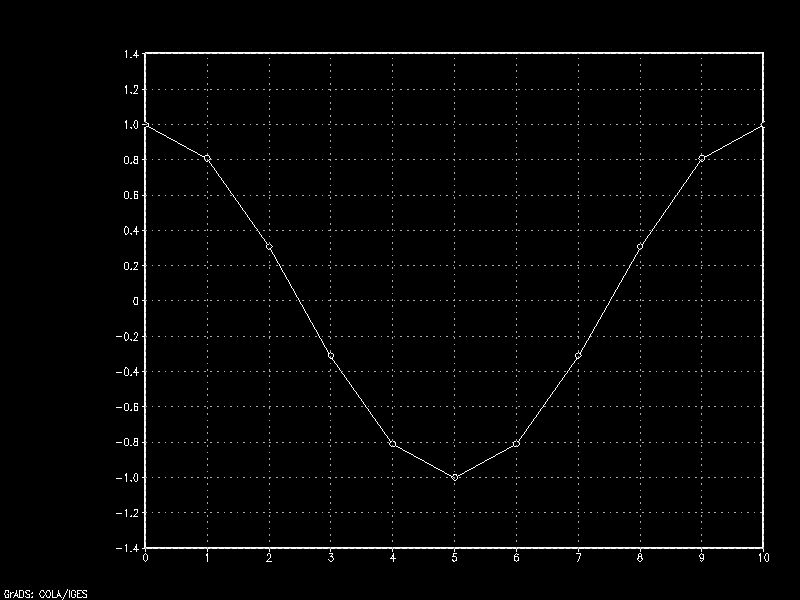
It looks like ^^ this given a wavelength \(n\) of 10. We can begin solving the partial derivative on the right-hand-side of equation (1) above using a finite differencing through space. The most basic way to approach a solution is to start with an upstream scheme. That means we’ll look backward through space some \(\Delta x\). For ease, that distance will be one meter.
Plugging the values of \(\psi\) at x=0 (1) and x=1 (0.809), a solution for the derivative of \(\psi\) with respect to \(x\) at time t=0 is:
$$\Target{e.1} (for \ x=1): {\partial \psi \over \partial x} = {0.809 – 1 \over 1} = -0.191$$
The example above can be parameterized using the notation shown below:
$$\Target{3} {\partial \psi \over \partial x} = {\psi ^n _i – \psi ^n _{i-1} \over \Delta x}$$
Subscript \(i\) of \(\psi _i\) denotes the direction of finite differencing through space.
$$\underset{x=0} {\psi ^n _{i-1}} \quad\text{ }\quad \underset{x=1} {\psi ^n _i} \quad\text{ }\quad \underset{x=2} {\psi ^n _{i+1}}$$
Shown above, \(\psi _i\) refers to the the value of \(\psi\) at x=1. \(\psi _{i-1}\) refers to the value of \(\psi\) one grid point to the left at x=0. Conversely, \(\psi _{i+1}\) refers to the value of \(\psi\) \(1 \Delta x\) to the right of \(\psi _i\) at x=2.
Okay, now that we’ve covered the spatial derivative on the right-hand-side of equation (1), let’s talk about the partial derivative on the left-hand-side, which accounts for the change of \(\psi\) through time. If we can find a solution for it, we will be able to solve for future values of \(\psi\). This is where things get really interesting. You with me?
Solving through time
$$\Target{4} {\partial \psi \over \partial t} = {\psi ^{n+1} _i – \psi ^n _i \over \Delta t}$$
Similar to how we use subscript \(i\) to solve derivatives through space, superscript \(n\) of \(\psi ^n\) defines the direction of finite differencing through time. \(\psi ^n\) holds the value of \(\psi\) at the present time. \(\psi ^{n-1}\) holds the value of \(\psi\) one time step in the past. \(\psi ^{n+1}\) represents the value of \(\psi\) one time step into the future. A simple one step forward-through-time difference shown in equation (4) above will be used for our approach below.
Substituting equations (3) and (4) into (1) above, we arrive at:
$$\Target{5} {\psi ^{n+1} _i – \psi ^n _i \over \Delta t} = -c{\psi ^n _i – \psi ^n _{i-1} \over \Delta x}$$
Solving for \(\psi ^{n+1} _i\) in the above equation yields the value of \(\psi\) at point \(i\) one step forward in time.
$$\Target{6} {\psi ^{n+1} _i = \psi ^n _i -c{\Delta t \over \Delta x}(\psi ^n _i – \psi ^n _{i-1})}$$
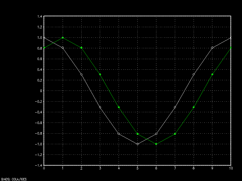
Given a wave propagation speed \(c\) of one meter per second, we can solve for \(\psi\) one second (\(\Delta t\)) from now. Noting values of \(\psi\) at x=0 (1), x=1 (0.809), x=2 (0.309), and x=3 (-0.309):
$$\Target{e.2} (for \ x=1): {\psi ^{n+1} _i = 0.809 -1{1 \over 1}(0.809 – 1)} = 1$$
$$(for \ x=2): {\psi ^{n+1} _i = 0.309 -1{1 \over 1}(0.309 – 0.809)} = 0.809$$
$$(for \ x=3): {\psi ^{n+1} _i = -0.309 -1{1 \over 1}(-0.309 – 0.309)} = 0.309$$
Continuing in this way for all points \(x\) and plotting the new values obtained for \(\psi\) in green below, we see the affect of wind speed \(c\) as it advects the wave towards the right.
The true analytic solution for constant advection would be perfect amplitude preservation and phase speed conservation. Unfortunately, our simple forward-through time, backward-through-space (upstream) scheme is a first-order method. This means it only considers the first polynomial of the scheme’s Taylor series expansion. All the rest are truncated.
Though the sum of these truncated terms is small, the error grows ever larger with continued integration through time. The end result is wave dampening. We’ll see this in a bit below. And we will explore the use of some higher-order schemes to address this truncation error a little later.
Courant-Friedrichs-Lewy condition
As a general rule, given maximum speed of feature \(c\), it is unwise to choose values of \(\Delta t\) and \(\Delta x\) that do not satisfy the Courant-Friedrichs-Lewy (CFL) condition:
$$\Target{7} {\nu = {c \Delta t \over \Delta x} \leq 1}$$
When advection serves as the dominant method of dispersion, not adhering to the above CFL criteria may result in large inaccuracies and numerical instability. If this instability is large enough, the simulation will fail to converge on a solution and will produce wildly incorrect results.
Experienced modelers know how to find a balance between the parameters above. Many times, the maximum wind speed value \(c\) will determine the proper grid-scale and time step. It also depends on what features you are trying to study. Gravity waves, for instance, travel at the speed of sound.
You can lower the CFL number by tuning the time step \(\Delta t\) or grid size \(\Delta x\). Decreasing the time step will increase computational expense. Increasing grid size will decrease model resolution. You can change both of these to fit your particular needs.
All of the model runs for the schemes shown below are tuned with CFL numbers ranging from 0.7 to 0.9 to assure numerical stability.
Upstream finite differencing scheme
To review, equations (5) and (6) above correspond to a first-order forward in time, backward in space (upstream) finite differencing scheme. They are:
$${\psi ^{n+1} _i – \psi ^n _i \over \Delta t} = -c{\psi ^n _i – \psi ^n _{i-1} \over \Delta x}$$
$${\psi ^{n+1} _i = \psi ^n _i -c{\Delta t \over \Delta x}(\psi ^n _i – \psi ^n _{i-1})}$$
Solving for \(\psi ^{n+1} _i\) for all values \(x\) yields the wave \(\psi\) one time step into the future. Repeat the process using our new values and we solve for the wave at time step 2. Do it again and again and you have a numerical model forecast:
Though wave amplitude dampening is prevalent with successive time steps, the speed of wave propagation is fairly accurate using this scheme. In reality, however, this upside is more or less moot.
Because this method looks in one direction only (backward in space), it cannot handle any change in the direction of advection (ie: a wind blowing from right to left across our model domain). This simple scheme largely serves us as a platform to examine more complex higher-order methods.
Higher-order finite differencing
Looking spatially in only one direction is not practical for studying real-world, multi-directional systems. Having the ability to look in other directions is essential. And it also contains a surprising feature. It reduces the amount of error introduced by truncating higher-order terms. Here, I’ll show you. Consider a Taylor series expansion of equation (3) above:
$${\Target{8} {\partial \psi \over \partial x} = {\psi ^n _i – \psi ^n _{i-1} \over \Delta x} \color{grey}{+ \geq 2nd–order \ terms}}$$
$${\Target{9} \psi ^n _{i-1} = \psi ^n _i – \Delta x {\partial \psi \over \partial x} \color{grey}{+ {1 \over 2!} \Delta x ^2{\partial ^2 \psi \over \partial x ^2} – {1 \over 3!} \Delta x ^3{\partial ^3 \psi \over \partial x ^3} + {1 \over 4!} \Delta x ^4{\partial ^4 \psi \over \partial x ^4} …}}$$
As stated previously, the first of the higher-order truncated terms (shown in gray) is the second derivative, making this backward in space scheme first-order accurate. Now we’ll extend this approach in the opposite direction, forward in space:
$${\Target{10} {\partial \psi \over \partial x} = {\psi ^n _{i+1} – \psi ^n _i \over \Delta x} \color{grey}{+ \geq 2nd–order \ terms}}$$
$${\Target{11} \psi ^n _{i+1} = \psi ^n _i + \Delta x {\partial \psi \over \partial x} \color{grey}{+ {1 \over 2!} \Delta x ^2{\partial ^2 \psi \over \partial x ^2} + {1 \over 3!} \Delta x ^3{\partial ^3 \psi \over \partial x ^3} + {1 \over 4!} \Delta x ^4{\partial ^4 \psi \over \partial x ^4} …}}$$
Subtract equation (9) from equation (11) and we come to:
$${\Target{12} \psi ^n _{i+1} – \psi ^n _{i-1} = 2 \Delta x {\partial \psi \over \partial x} \color{grey}{+ {2 \over 3!} \Delta x ^3{\partial ^3 \psi \over \partial x ^3} + {2 \over 5!} \Delta x ^5{\partial ^5 \psi \over \partial x ^5} …}}$$
Note the odd numbered terms of (9) and (11) have canceled out. Note too the first of the higher-order truncated terms is the third derivative. This makes this centered in space scheme second-order accurate, an improvement over the first-order accuracy of the upstream scheme.
Expressing this equation in terms of \({\partial \psi \over \partial x}\), we arrive at:
$${\Target{13} {\partial \psi \over \partial x} = {\psi ^n _{i+1} – \psi ^n _{i-1} \over 2 \Delta x} \color{grey}{+ \geq 3rd–order \ terms}}$$
Let’s take a look at some more sophisticated schemes.
Heun Runge-Kutta finite differencing scheme
Here is a second-order Runge-Kutta forward-in-time, centered-in-space finite differencing scheme with coefficient values \(a _1\) and \(a _2\) specified by Heun.
$$\psi ^{n+1} _i = \psi ^n _i + (a _1 k _1 + a _2 k _2)h$$
$$a _1 = {1 \over 2} \ ; \ a _2 = {1 \over 2} \ ; \ h = \Delta t$$
$$k _1 = f(x _i, \psi ^n _i)$$
$$k _2 = f(x _i + h, \psi ^n _i + k _1 h)$$
$${\Target{14} \psi ^{n+1} _i = \psi ^n _i – c{\Delta t \over 4 \Delta x}(\psi ^n _{i+1} – \psi ^n _{i-1})}$$
This approach first approximates \(\partial \psi \over \partial x\) at the current time step (\(k _1\)), and then \(\partial \psi \over \partial x\) at the next time step (\(k _2\)). It then finds how \(\psi\) varies through space and time by averaging slopes \(k _1\) and \(k _2\). It predicts the value of \(\psi _i\) at the next time step using this average slope.
Our wave amplitude dampening problem is no more. The wave actually grows in amplitude – also a problem. This could be improved with higher grid resolution. This scheme also drastically reduces wave advection speed. That’s not untypical for the scheme.
The example below shows the results of high advection speed and only moderate spatial resolution where instability breaks the wave apart.
Adams-Bashforth finite differencing scheme
Below is a second-order accurate Adams-Bashforth time scheme with centered in space differencing.
$${\psi ^{n+1} _i – \psi ^n _i \over \Delta t} = -c[{3 \over 2}({\psi ^n _{i+1} – \psi ^n _{i-1} \over 2 \Delta x}) – {1 \over 2}({\psi ^{n-1} _{i+1} – \psi ^{n-1} _{i-1} \over 2 \Delta x})]$$
$${\Target{15} \psi ^{n+1} _i = \psi ^n _i – c{\Delta t \over 4 \Delta x}[3(\psi ^n _{i+1} – \psi ^n _{i-1}) – (\psi ^{n-1} _{i+1} – \psi ^{n-1} _{i-1})]}$$
While prior schemes above solve for and then throw away calculations from previous time steps, this multistep method retains past values. This works intuitively and mathematically. Knowing more about the behavior of a function in the past can help to determine what the function may do in the future. Since these calculations have already been performed, the value added can easily offset the relatively small computational expense of holding the additional memory.
Another advantage of using the Adams-Bashforth method over the Runge-Kutta methods is that only one evaluation of the integrand f(x,y) is performed for each step. It should be noted, however, that this scheme is especially sensitive to high CFL values as the example below attests.

Leapfrog finite differencing scheme
Here is a second-order scheme that is centered in time and centered in space.
$${\psi ^{n+1} _i – \psi ^{n-1} _i \over 2 \Delta t} = -c{\psi ^n _{i+1} – \psi ^n _{i-1} \over 2 \Delta x}$$
$${\Target{16} \psi ^{n+1} _i = \psi ^{n-1} _i – c{\Delta t \over \Delta x}(\psi ^n _{i+1} – \psi ^n _{i-1})}$$
As with the other higher-order schemes, the Leapfrog scheme offers second-order accuracy by being centered in space. Like the Adams-Bashforth scheme, it retains past values. This comes naturally by being centered in time. This results in increased accuracy as we iteratively calculate future states.
Wave amplitude dampening is relatively minor and phase speed preservation is good for CFL values less than one. The major drawback to this scheme is its development of a bimodal solution. Unlike the previous schemes whose first term on the right-hand-side is self-referencing (\(\psi ^n _i\)), this method contains no such grounding. Instead, this scheme calculates the change of \(\psi\) by looking at current points to the left and right, as well as itself for the previous time step.
Essentially, the Leapfrog method splits the entire dataset into two camps: the odd grid points along x who respond to changes in the even grid points surrounding, and the even grid points similarly modified by their surrounding odd points. This decoupling physically manifests itself as a pulsating wave.
Leapfrog scheme with Asselin filter
The bimodal problem encountered with the Leapfrog scheme can be addressed by adding an Asselin filter. Check it.
$${\Target{17} \psi ^n _i = \psi ^n _i + a(\psi ^{n+1} _i – 2 \psi ^n _i + \psi ^{n-1} _i)}$$
Above, \(a\) is an Asselin coefficient constant. Applying the above equation on the just solved value of \(\psi\) at point \(x\) eliminates decoupling between even and odd horizontal x-grid points.
In effect, the Asselin filter adds guardrails and allows the Leapfrog scheme to converge on a single solution. The cost of adding this filter comes with weak suppression of the numerical solution. The animation shows slight wave amplitude dampening.
In the end, I chose the Leapfrog finite differencing scheme with Asselin filtering for my mesoscale model. Its easy implementation, numerical stability (even at CFL numbers approaching 1), computational thrift, and relatively low run-time storage requirements ultimately made it the method of choice.